Bellman's Curse
Seconds after I wrote this title, as corny as it may be, I stumbled upon a Wikipedia subheading, Curse of dimensionality. In order to divert graduate students early, and to prevent scaring my targeted demographic, we're not in that deep yet. There shall not be any cursed phenomena occuring here!
Instead, I want to touch on dynamic programming, hereafter referred to as DP, a general problem solving approach coined by Richard Bellman in the 1950s to describe an optimization method in which larger problems are recursively broken down into simpler subproblems. To prevent the haunting of Bellman's brilliant mind, the only curse here is the general animosity from interviewees towards technical hiring challenges geared around dynamic programming. Why the loathing? Well, if you've tried a subset of dynamic programming problems, you've most likely found them, at first, non-intuitive. Additionally, DP is not a trick that you can learn to solve any DP problem. DP can take a couple forms - top-down with recursion and memoization, or bottom-up without memoization. Moreover, it is not trivial to recognize a problem on its own as solvable with a DP approach.
In order to lay out the details in my own head and provide a jumping board for tackling divide-and-conquer problems to DP challenges, I'll discuss the following:
- The difference between the divide-and-conquer and DP approaches
- The basis for recognizing DP problems
- Famous examples of DP problems (Knapsack, Chain Matrix, etc.)
First, many students often begin their education in algorithms with the divide-and-conquer technique. When I transitioned to learning dynamic programming, I found it difficult to separate the two problem solving approaches since both approaches lean towards recursively dividing the larger problem into smaller sub-problems. Then, both applications make use of the smaller subproblems by combining their results to achieve the optimal solution.
For instance, a great example of the divide-and-conquer technique is mergesort: In its usually elementary implementation, Mergesort works by recursively dividing a list into n sublists. Then, each unit in a sublist is merged against sister sublists to produce new sorted sublists until the entire list has been sorted. The pseudocode of Mergesort is provided below without the implementation of the merge routine - a comparison routine used to sort and merge adjacent lists:
def mergesort(A: list, low: int, high: int):
    if low < high:
        middle = low + ((high - low) / 2)
        mergesort(A, low, middle)
        mergesort(A, middle + 1, high)
        merge(A, low, middle, high)
As shown above, mergesort sorts a list of size n by recursively sorting two sublists of size n/2. Thus, the subproblem size is substantially smaller than original problem size. In mergesorts case, the larger problem is halved at each recursive division, so the recursion tree has only logarithmic depth and a polynomial number of nodes.
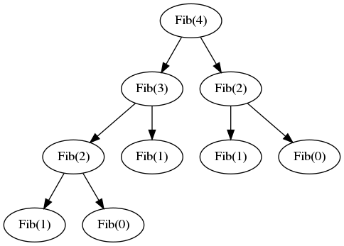
In contrast, typical DP approaches are solved by building on slightly smaller subproblems. In the Knapsack problem, explained further on down, we're given n items to store in a bag with a capacity of at most W pounds. In order to make sure the capacity hasn't been fulfilled, a solution would have to keep track earlier subproblem results. Thus, the full recursion tree generally has polynomial depth and an exponential number of nodes resembling something like a Fibonacci series progression as shown below:
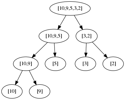
Additionally, the divide-and-conquer approaches focus on subproblems that are independent of each other. In the Mergesort Division figure above, sorting [3,2] does not rely on [10,9,5] already being sorted. A merge routine will take care of the sorting and merging, but the merge routine can sort the sublists independently; consequently, the mergesort makes a decent case for natually splitting the work that can be run in parallel. As seen in the Knapsack case,a DP approach arrives to a solution by combining earlier dependent results. The decisions of K(i), whether to accept a weighted item, depend on the result of K(i - 1) since the capacity might have been reached.
Identifying DP-approachable Problems
So, how do I know to apply DP when I see a problem?
Dynamic Programming is a technique of very broad applicability, but problems solvable with a DP approach can manifest in several forms:
- Can the larger problem be broken down into smaller subproblems worth caching?
- Optimization problems: What is the minimum/maximum, fewest/greatest, longest/shortest, etc?
Regarding the first point, divide-and-conquer and DP overlap. Should sorting a list of elements be approached through DP? Of course not. Refer to my earlier point of recognizing dependence of a subproblem solution. Sorting requires no dependence when operating at the subproblem level (i.e. you can sort three objects without knowning about the rest of the objects in the list.) Furthermore, is it apparent that the same suproblem is being solved multiple times? For large numbers N, the Fibonacci series diverts to solve smaller subproblems repeatedly. In our example, Fib(1) is attempted thrice. In a DP approach, we can calculate Fib(1) once, stores its result in a cache, and query the cache as a constant time operation when the result is necessary.
Second, DP-approachable problems usually ask a question in the form of reaching a mathematical optimization. As examples, in Algorithms [Dasgupta, Papamdimitriou, Vazirani], problems range from finding the longest increasing subsequence in a list of integers, determining the optimal order of chain matrix multiplicatons to minimize multiplications, and finding the shortest path from a starting node to an ending node.
A Famous DP Example
Touched on earlier, the Knapsack problem is a quintessiential problem used to teach DP. The general problem revolves around making a decision on whether to insert a weighted object into a knapsack with capacity W. As another constraint, these weighted objects are valued differently so it's possible that an object weighing 10 pounds may only be valued at $5 whereas another object weighing 2 pounds may be valued at $30. An example input is shown below:
| Item | Weight | Value |
|---|---|---|
| 1 | 7 | $3 |
| 2 | 4 | $10 |
| 3 | 10 | $4 |
| 4 | 2 | $16 |
| 5 | 15 | $21 |
What is the most valuable combination of items we can fit into the knapsack without overflowing our capacity?
We'll approach the Knapsack problem (and most DP problems) by:
- Defining the subproblem
- Defining the recurrence relation for those subproblems
The method defined above works well for most DP-approachable problems. It's easier to grasp the construction of the solution by defining a subproblem. Once the subproblem is defined, dependencies can be established between other subproblems so that an optimal solution is revealed.
For this instance of the problem, we'll not be constained by the possible combination of items (i.e. we can pick the same item multiple times). For a capacity of 10 pounds, we can start by taking item 1 with a weight of 7. Our total capacity drops to 3 pounds so we have only one more choice which happens to be item 4. No other items fit into our knapsack so we have our final solution for a total value of $3 + $16 = $19. However, it's obvious that the combination of item 1 and item 4, the greedy approach, is not the optimal solution. In fact, the combination of item 4 multiple times leads to the optimal solution since item 4 maximizes value without overtaxing the capacity.
Since we're able to use objects multiple times, it becomes apparent that we don't need to keep track of what object is inserted into our knapsack. A DP-approach would be to build up a one-dimension table of length W + 1 where each item is evaluated of the current capacity w.
At every evaluation of the pool of objects for the current capacity of w, we must ensure that an insertion into our knapsack won't overflow the capacity. Thus, when choosing an item, we must choose the item that is most valuable and will not break our capacity limit. Thus, we've defined our subproblem - K(w) is the maximum valuable item i from the multiset of items {1, ..., i} achievable with a knapsack of capacity w.
The problem, defined above, is resolved dependent on smaller subproblems until the full capacity W is reached or there are no items left in the pool of objects that would not overflow the capacity. For instance, when evaluating K(w) for item i, we must choose whether there exists an item i so that item i will provide the optimal solution dependent on our previous choices so that our capacity doesn't overflow. Thus, our recurrence relation is constructed as following: - K(w) = max {K(w - wi) + vi} where wi and vi are the weight and value of item i respectively.
The full solution is provided below in code:
def maximum_valuable(weights: list, values: list, B: int):

  # Initialize a 1D table of length B + 1
  # to hold the capacities
  K = [0 for idx in range(0, len(B) + 1)]

  # Let w be the current capacity of the total
  # capacity B, build the table K where we
  # evaluate smaller capacities first
  for w in range(0, B):
    # Find the maximum valuable item i
    # for a capacity w and set K(w)
    for index,weight in enumerate(weights):
      if weight <= w and K(w) < K(w - weight) + values[index]
        K[w] = K(w - weight) + values[index]

  # Since our table is built up from smaller
  # capacities, the last entry should have the
  # combination of the most valuable items of
  # capacity B
  return K[B]